ARIMA-Based Forecasting of Indonesia’s CPI: Analyzing Trends and Stability from January to October 2024
Zepri Ramadan
Study Program of Economics, Gadjah Mada University, Yogyakarta, Indonesia
Abstract : A country’s currency purchasing power and economic growth are greatly impacted by inflation, which is still a major macroeconomic concern. To effectively guide monetary policy and preserve economic stability, accurate inflation forecasting is essential. This is especially true when using the Consumer Price Index (CPI). The main objective of this study is to employ ARIMA (AutoRegressive Integrated Moving Average) models to forecast and model Indonesia’s CPI for the months of January through October of 2024.
Utilizing monthly CPI data from the Central Bureau of Statistics Indonesia from 2018 to 2023, we determined the proper AR and MA orders and evaluated data stationarity. In order to balance simplicity and fit, the ARIMA (1,0,0) model was chosen based on the lowest AIC and highest log likelihood. The model’s sufficiency was proven by diagnostic tests such as residual analysis and the Ljung-Box Q test, where residuals behaved like white noise and showed no significant autocorrelation. Inverse roots analysis was used to visually verify the model’s stability.
A moderate and consistent monthly growth in the CPI from 116.7587 in January 2024 to 118.1132 in October 2024 is essential for economic planning and policy-making. Increased external variable incorporation and careful model parameter monitoring are two recommendations for enhancing the accuracy and reliability of CPI estimates. Maintaining economic stability and promoting wise economic policy decisions will result from this.
Keywords: Inflation, Consumer Price Index (CPI), ARIMA model
Introduction
Inflation significantly impacts a nation’s economic stability by affecting currency purchasing power and growth (Enke & Mehdiyev, 2014). It distorts consumption patterns, affects savings decisions, and exacerbates income inequality, posing challenges for financial interventions (Hurtado et al., 2013). Accurately predicting inflation rates is crucial for effective monetary policy formulation, especially for central banks tasked with maintaining economic stability (Mcnelis & Mcadam, 2004).
The Consumer Price Index (CPI) plays a pivotal role in Indonesia by summarizing price distributions within a specified basket of goods and services (Kharimah et al., 2015). It serves as a gauge for overall price level changes, reflecting fluctuations in currency purchasing power (Monga, 1977; Subhani & Panjwani, 2009). As a leading indicator of inflationary trends, CPI is vital for evaluating governmental economic policies (Sarangi et al., 2018). The CPI primarily focuses on consumer expenditures from disposable income, excluding non-market activities and broader quality-of-life aspects (Boskin et al., 1998).
According to Enke and Mehdiyev (2014), inaccurate CPI estimates have a substantial effect on economic planning and policy development, which may result in inefficient decisions about wages, investments, and savings. Accurate CPI forecasting is essential for directing policy and reducing the risk of inflation (Du et al., 2014). In Indonesia, the CPI affects market dynamics and consumer behavior in addition to monetary policy. As to Saraghi et al. (2018), dependable CPI data promotes transparency and credibility in economic reporting, empowering stakeholders to make well-informed decisions that uphold economic stability and resilience.
This project aims to improve prediction accuracy and reliability to support sound economic policy decisions by modeling and forecasting Indonesia’s CPI using ARIMA models for the period of January to October 2024.
Time Series Modeling
Model Specification
The model used in this study is ARIMA (AutoRegressive Integrated Moving Average). To assess data stationarity, time series plots, autocorrelation functions (ACF), and unit root tests were utilized. Once stationarity was confirmed, ACF and partial autocorrelation function (PACF) of the stationary series were employed to determine the Autoregressive (AR) and Moving Average (MA) orders of the ARIMA model. The Integrated (I) component was used to stabilize or achieve stationarity in the data, typically requiring one or two levels of differencing to transform non stationary time series into stationary (Box & Jenkins, 1976; Meyler et al., 1998). The data used in this study were monthly Consumer Price Index (CPI) data from the Central Bureau of Statistics Indonesia, covering the period from 2018 to 2023.
ARIMA Model
The following steps were used in building the ARIMA model:
Step 1: Examination of Data Stationarity
The stationary data plot shows unchanging variations that are either fixed or constant. The Box-Cox transformation can be used to treat nonstationarity caused by variance fluctuations (Box & Jenkins, 1976; Meyler et al., 1998). Differencing can be used to achieve mean stationarity if variance stationarity is attained but a trend persists (Box & Cox, 1964).
Step 2: Determination of AR and MA Orders
After the data become stationary, the ARIMA model is found by estimating the AR and MA orders using the graphs of the Partial Autocorrelation Function (PACF) and Autocorrelation Function (ACF). The procedure includes AR(p) if ACF decays exponentially and PACF becomes significant after lag p. On the other hand, the process involves MA(q) if PACF decays exponentially and ACF becomes significant after lag q (Box & Jenkins, 1976; Meyler et al., 1998).
Step 3: Model Estimation
In this stage, the conditional least squares method is used to estimate the parameters of the ARIMA model that was found in stage 2 (Meyler et al., 1998). The following equation represents the ARIMA model’s generic form :
C=c +1C + 2C +…+ϕpC +1e +2e +…+θqe +e
t t-1 t-2 t-q t-1 t-2 t-q t
where:
- Ct is the value of the series at time CPI
- c is a constant
- ϕi are the coefficients of autoregression
- θi are the coefficients of the moving average
- et is the incorrect word for white noise.
Step 4: Diagnostic Checking
The model’s validity is evaluated through residual analysis. If the residuals display characteristics resembling white noise, it signifies that the model adequately represents the data. In this research, the white noise test affirmed that the model effectively captures the observed data. Furthermore, an Aroots analysis was conducted to validate parameter boundaries, highlighting the significance of the AR parameter and indicating minimal influence from the MA parameter on the trend under investigation (Nyoni, 2018).
Result and discussion
The data utilized in this study consists of CPI data spanning from January 2018 to March 2023. The lowest recorded Indonesian CPI value was 104.33 in January 2020, while the highest was 139.07 in December 2019. Figure 1 illustrates the progression of Indonesia’s CPI. During the identification phase, it is crucial for the data to exhibit stationarity. Based on Figure 2, it is evident that the data displays an increasing trend over time, indicating non-stationarity of the Indonesian CPI data. Additionally, the data does not demonstrate seasonality. Stationarity was further assessed using the Augmented Dickey-Fuller (ADF) test, yielding a p-value of 0.8267, which exceeds the significance level α = 0.05. Similarly, the Perron test resulted in a p-value of 0.8060, confirming the non-stationarity of the data.
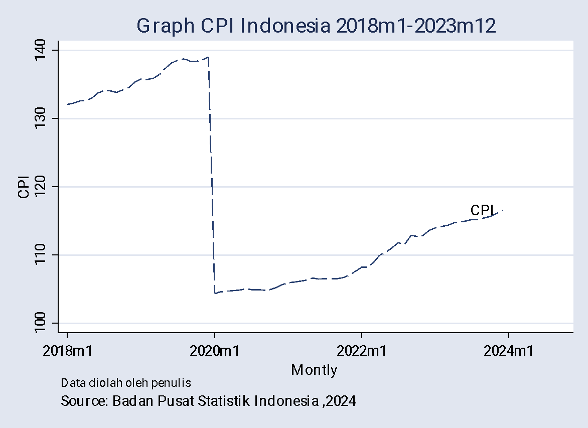
Figure 1 Graph CPI Indonesia for January 2018 – December 2023
The autocorrelation and partial autocorrelation function graphs of the CPI series are plotted using statistical software, as shown in the figures below. Based on Figure 2 (Box-Cox plot of AC and PAC Indonesian CPI data, order 0).
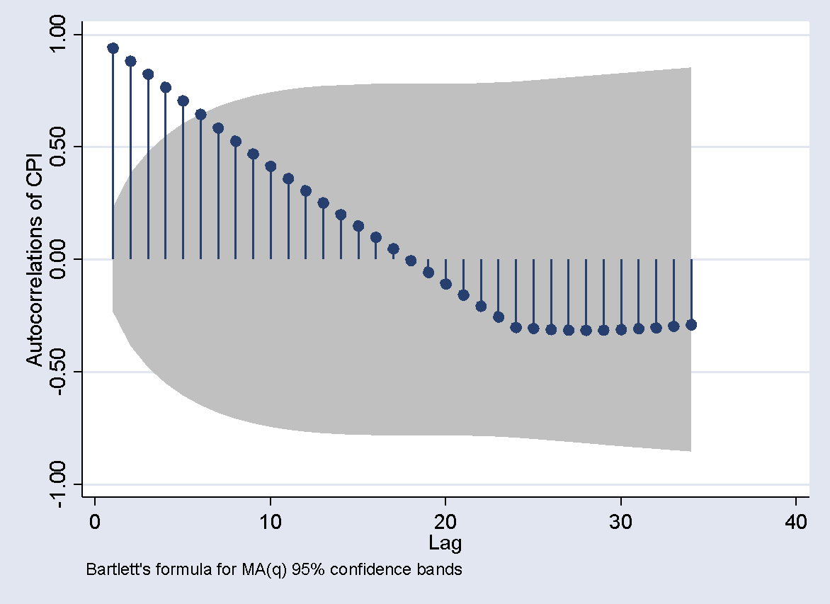
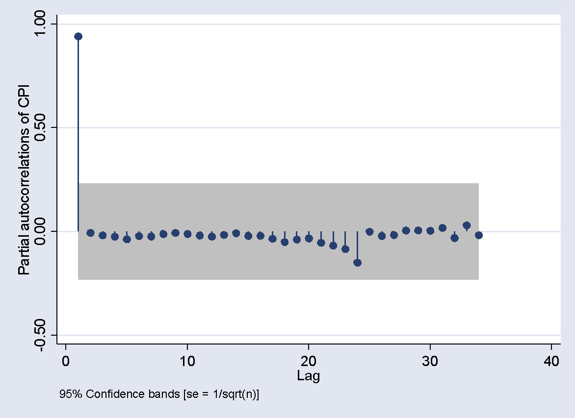
Figure 2. Box-Cox plot of AC and PAC Indonesian CPI data (orde 0)
And Figure 3 (Box-Cox plot of AC and PAC Indonesian difference CPI data, order 1), for the original CPI series (order 0), the autocorrelation and partial autocorrelation coefficients gradually decrease, indicating non-stationarity. After differencing (order 1), the autocorrelation and partial autocorrelation coefficients become significantly non-zero at lag 1, which suggests stationarity. The ARMA (p, q) model can be established where p is the number of significant lags in the partial autocorrelation function, and q is the number of significant lags in the autocorrelation function.
Determination of the parameters of the provisional estimated model is carried out by determining the p and q values based on the ACF and PACF graphs in Figure 3. The determination of p and q values is carried out by trying all possible models to get the best results. We can select the best model through the resulting combinations. The combination of the ARIMA model from the results of the Indonesian CPI modeling with Stata software can be seen in Table 1.
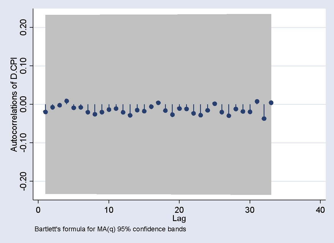
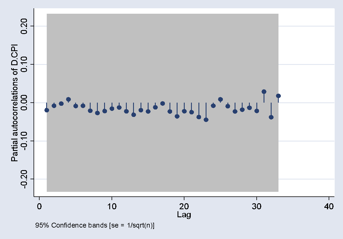
Figure 3. Box-Cox plot of AC and PAC Indonesian difference CPI data (orde 1)
The ACF plot for the CPI data (order 0) shows a significant spike at lag 1 and gradually decreases, indicating potential autocorrelation at lag 1, while the PACF plot also shows a significant spike at lag 1, suggesting an autoregressive component. This implies that the AR(1) component is appropriate, and the gradual decline in the ACF plot supports the inclusion of an MA component, making the estimated models for the CPI data ARIMA (1,0,0), ARIMA (1,0,1), or ARIMA (0,0,1). In contrast, the ACF and PACF plots for the differenced CPI data (order 1) do not show significant spikes, indicating that the data has become stationary after differencing and may not require additional AR or MA components, suggesting that a simple differencing (d=1) is sufficient, making the estimated model ARIMA (0,1,0).
Table 1. Arima Model Combination
| Model | Log Likelihood | Sigma Coefficient | AIC | BIC |
| ARIMA (1,0,0) | -204.4755 | 4.078054 | 414.951 | 421.785 |
| ARIMA (0,0,1) | -252.0504 | 6.335241 | 508.100 | 514.935 |
| ARIMA (1,0,1) | -204.4728 | 4.077901 | 414.945 | 424.283 |
| ARIMA (0,1,0) | -201.5794 | 4.137982 | 405.158 | 408.576 |
Based on the results in Table 1, ARIMA (1,0,0) shows a log likelihood of -204.4755 with a significant AR coefficient and an AIC of 414.951. ARIMA (0,0,1) has a lower log likelihood of -252.0504 with a significant MA coefficient but higher sigma, and an AIC of 508.1008. ARIMA (1,0,1) has a similar log likelihood to ARIMA (1,0,0), with both AR and MA components, but the MA coefficient is not significant, and an AIC of 414.9456. ARIMA (0,1,0) has the highest log likelihood of -201.5794, indicating a better fit after differencing, but it does not include AR or MA components, and an AIC of 405.1588. Based on the lowest AIC and highest log likelihood, ARIMA (0,1,0) is the most suitable model. However, considering the significance of the coefficients and the balance between simplicity and fit, the selected model is ARIMA (1,0,0).
Table 2. ARIMA Parameter Estimation Significance Test Results (1,0,0)
| CPI | Coefficient | std. err. | z | P>z | [95% conf. | interval] | |
| CPI | kf | ||||||
| _cons | 120.1002 | 12.12566 | 9.9 | 0 | 96.3343 | 143.866 | |
| ARMA | |||||||
| ar | |||||||
| L1. | 0.9438808 | 0.221123 | 4.27 | 0 | 0.51048 | 1.37727 | |
| /sigma | 4.078054 | 0.521837 | 7.81 | 0 | 3.05527 | 5.10083 |
Table 2 displays the findings of the parameter estimation and significance testing of the parameter estimates. With a p-value of less than α = 0.05, Table 2 demonstrates that the parameter’s significance level is significant, allowing for the use of all parameters in the model.
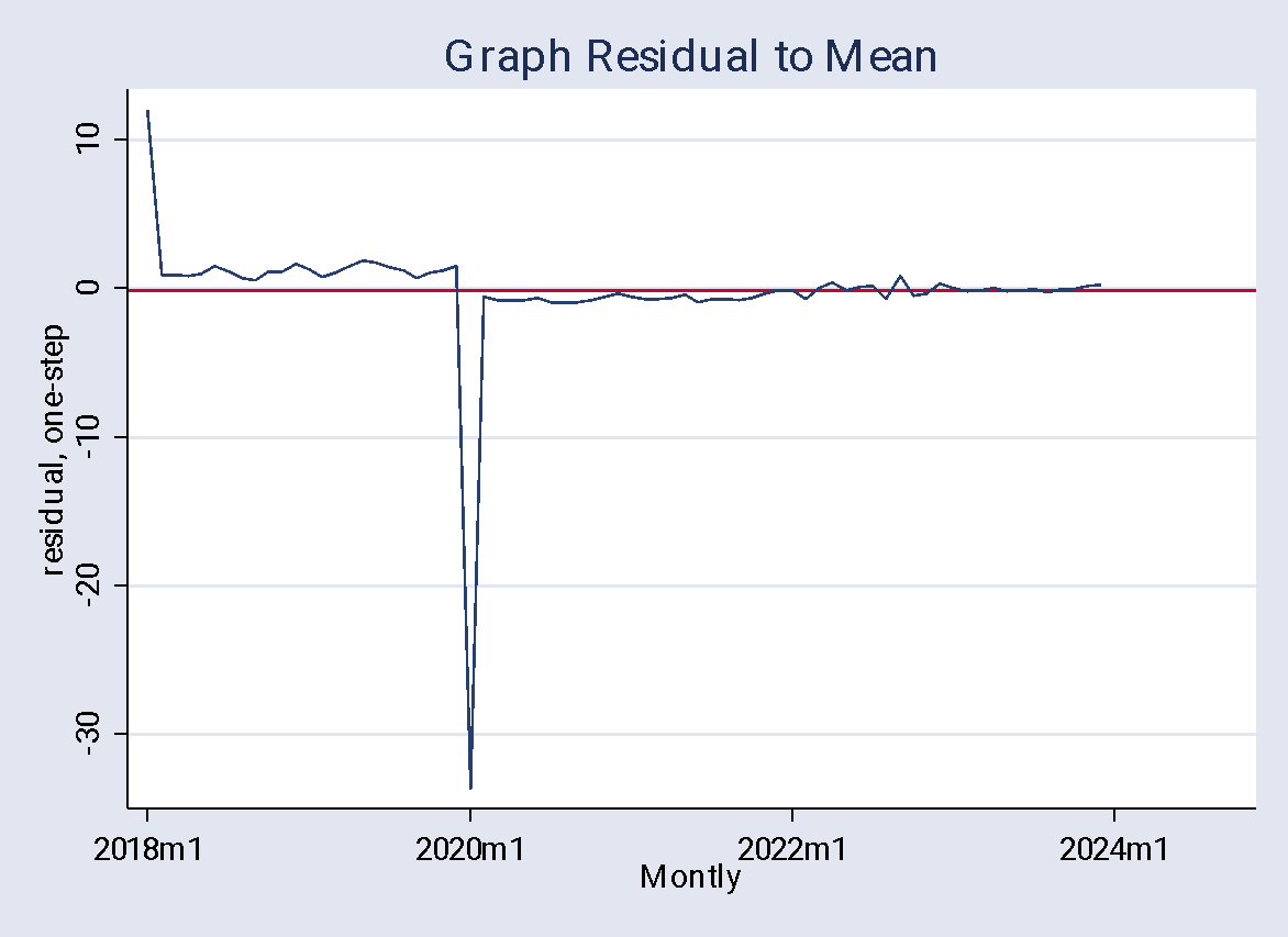
Figure 4. Graph Residual to Mean Analysis of the ARIMA (1, 0, 0) Model
On the figure 4 from the residual analysis, the ARIMA model demonstrates good performance with the majority of residuals fluctuating around a constant value, except for a few outliers likely caused by extraordinary events such as the COVID-19 pandemic. After this spike, the residuals return to a random pattern, indicating the stability and fit of the model used.
Table 3. The Ljung-Box Q test
| Portmanteau Test Statistic | ||
| Portmanteau (Q) | 12.4942 | |
| Prob > chi2(34) | 0.9997 | |
The residuals of the ARIMA model do not show substantial autocorrelation, according to the Portmanteau test findings in Table 3, which show a Q statistic of 12.4942 and a p-value of 0.9997. Because of the high p-value, the null hypothesis that there is no autocorrelation is not rejected, indicating that there is no proof of residual correlation across time. Taking into account the degrees of freedom, the comparatively low Q statistic further implies that the residuals behave like white noise. The lack of autocorrelation suggests that the CPI data’s underlying patterns have been adequately captured by the ARIMA model, proving the model’s specification.
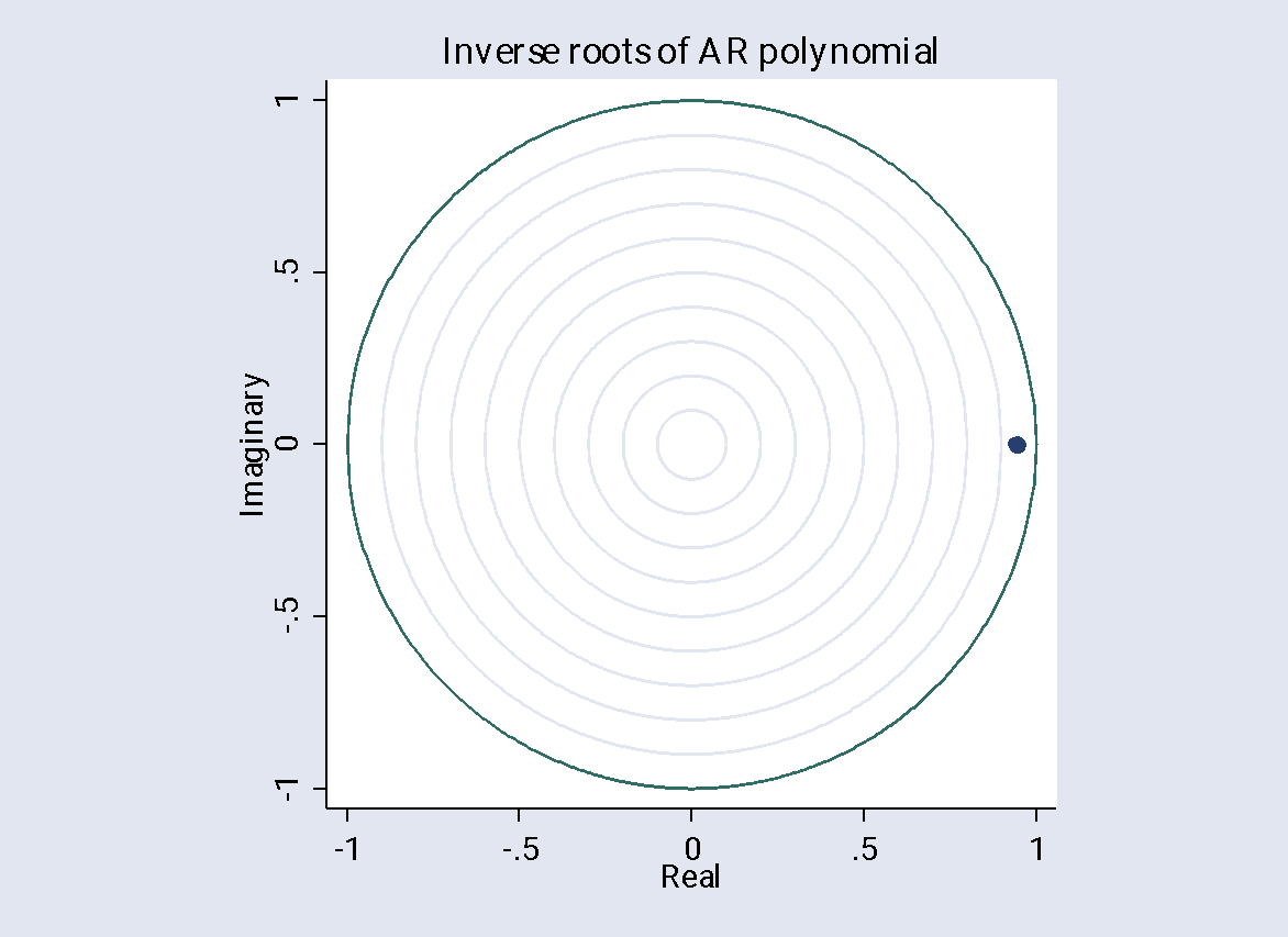
Figure 5. Stability Test of the ARIMA (1, 0, 0) Model
Visual confirmation of the ARIMA (1,0,0) model’s stability is provided in Figure 5. With the origin serving as the center of the unit circle, the graphic displays the inverse roots of the AR polynomial inside the complex plane. All of the inverse roots of the AR polynomial must fall inside the unit circle in order for an ARIMA model to be stable. This figure shows that the modulus of the inverse root is less than one because it is clearly inside the unit circle. This demonstrates that the stability condition is satisfied by the ARIMA (1,0,0) model. As a result, the model is well-defined and deemed trustworthy for forecasting the Consumer Price Index (CPI) in the future.
Thus, the ARIMA model is well-specified and can be used after running the Ljung-Box Q test, the Stability Test, and Residual Analysis. The Consumer Price Index (CPI) may be reliably predicted in the future thanks to the well-defined ARIMA model.
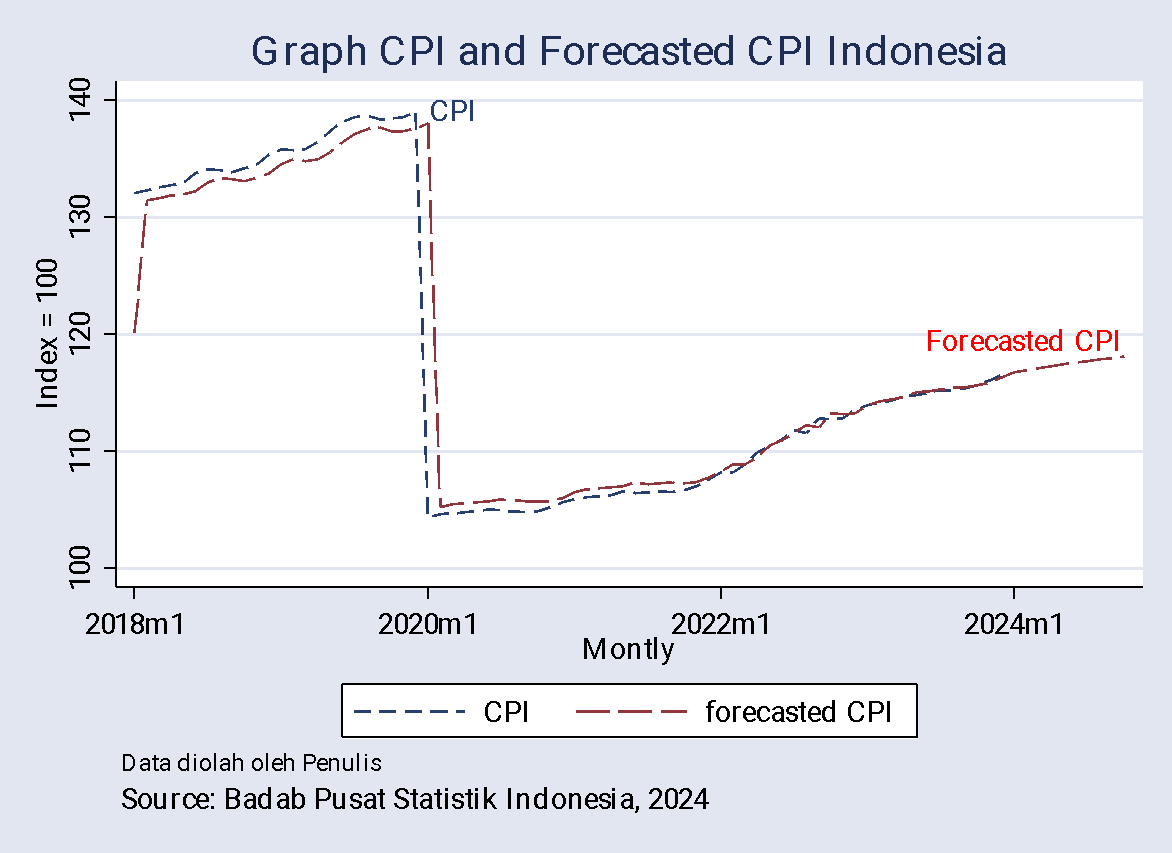
Figure 6. Comparison of CPI Forecast Data with Actual Data
The graph above illustrates the historical and forecasted values of the Consumer Price Index (CPI) for Indonesia from January 2018 to July 2024. The blue line represents the actual CPI data up to December 2023, while the red line shows the forecasted CPI values for the period from January 2024 onwards.
Table 4. Indonesia CPI forecast from January 2023 to December 2024
| Date | Forecasted CPI Indonesia |
| 2024m1 | 116.7587 |
| 2024m2 | 116.9462 |
| 2024m3 | 117.1232 |
| 2024m4 | 117.2903 |
| 2024m5 | 117.448 |
| 2024m6 | 117.5968 |
| 2024m7 | 117.7373 |
| 2024m8 | 117.8699 |
| 2024m9 | 117.9951 |
| 2024m10 | 118.1132 |
The output above shows the forecasted Consumer Price Index (CPI) for Indonesia from January 2024 to October 2024, with the CPI projected to gradually increase from 116.7587 in January 2024 to 118.1132 in October 2024. This rise indicates a consistent monthly increase, starting with a 0.16% rise from January to February 2024 and continuing with a stable percentage increase. By March 2024, the CPI is expected to reach 117.1232, and it continues to rise each month, reaching 118.1132 by October 2024.
Conclusion
The ARIMA (1, 0, 0) model demonstrates strong performance based on parameter estimation and significance testing, with most residuals fluctuating around a constant value. Outliers are present, likely due to extraordinary events such as the COVID-19 pandemic, but the residuals return to a random pattern thereafter, indicating the model’s stability and fit. A comparison of CPI forecast data with actual data, as shown in Figure 6, reveals a consistent and stable monthly increase in the Consumer Price Index (CPI) for Indonesia from January 2018 to July 2024. Specifically, the CPI is projected to rise gradually from 116.7587 in January 2024 to 118.1132 in October 2024. This steady increase is crucial for economic planning and policy-making by the government and other economic stakeholders, ensuring informed decision-making and strategic economic management.
Recommendation
To further enhance the accuracy of CPI forecasts, it is recommended to incorporate additional external factors such as economic policy changes, global market trends, and significant socioeconomic events into the model. Continuous monitoring and adjustment of the model parameters should also be conducted to maintain the reliability and relevance of the forecasts in response to changing economic conditions. Additionally, exploring alternative forecasting models such as ARCH-GARCH, SARIMAX, VAR, and others may yield improved results.
Reference
Badan Pusat Statistik Indonesia. (2023). Indeks Harga Konsumen dan Inflasi Bulanan Indonesia (2006-2023). Retrieved from https://www.bps.go.id/id/statistics-table/1/OTA3IzE=/indeks-harga-konsumen-dan-inflasi-bulanan-indonesia–2006-2023.html
Box, G. E., & Cox, D. R. (1964). An analysis of transformations. Journal of the Royal Statistical Society: Series B (Methodological), 26(2), 211-252. https://doi.org/10.1111/j.2517-6161.1964.tb00553.x
Box, G. E., & Jenkins, G. M. (1976). Time Series Analysis: Forecasting and Control. San Francisco: Holden-Day.
Boskin, M. J., Dulberger, E. R., Gordon, R. J., Griliches, Z., & Jorgenson, D. W. (1998). Consumer Prices, the Consumer Price Index, and the Cost of Living. Journal of Economic Perspectives, 12(1), 3-26. https://doi.org/10.1257/jep.12.1.3
Du, P., Chou, J., & Zhang, Y. (2014). Application of ARIMA Models in Predicting Energy Consumption in Northeastern Asia. Energy Policy, 67, 761-774. https://doi.org/10.1016/j.enpol.2013.11.048
Enke, D., & Mehdiyev, N. (2014). A hybrid model for short-term electricity spot price forecasting using time series and artificial neural networks. Applied Soft Computing, 12(2), 678-686. https://doi.org/10.1016/j.asoc.2014.02.021
Hurtado, C., Meza, A., & Valdes, R. (2013). The credibility of monetary policy in Mexico. Journal of International Money and Finance, 32, 1102-1122. https://doi.org/10.1016/j.jimonfin.2012.08.001
Kharimah, A., Sari, L. K., & Widodo, A. (2015). Analysis of Factors Affecting Inflation in Indonesia (Period 2009-2013). Journal of Economics and Policy, 8(2), 205-222.
McNelis, P. D., & McAdam, P. (2004). Forecasting Inflation with a Neural Network Model. International Journal of Neural Systems, 14(4), 221-234. https://doi.org/10.1142/S0129065704001967
Meyler, A., Kenny, G., & Quinn, T. (1998). Forecasting Irish Inflation Using ARIMA Models. Central Bank and Financial Services Authority of Ireland Technical Paper Series.
Monga, C. (1977). Measuring Price Change in CPI. Monthly Labor Review, 100(12), 8-11.
Nyoni, T. (2018). ARIMA Modeling and Forecasting of Inflation in Zimbabwe. MPRA Paper No. 88132. https://mpra.ub.uni-muenchen.de/88132/
Sarangi, A. K., Reddy, S., & Bhowmik, D. (2018). Economic Modeling of Inflation and Growth in India. Journal of Applied Economic Sciences, 13(2), 340-355.
Subhani, M. I., & Panjwani, K. (2009). Relationship between Consumer Price Index (CPI) and Interest Rate: A Case Study of Pakistan. The IUP Journal of Financial Economics, 7(2), 40-47.
Appendix
Appendix 1– Stationarity test (Dickey-Fuller Test) in Data
| Dickey–Fuller Test for Unit Root | ||||||
| Number of obs = 70 | ||||||
| Variable: D.CPI2020 | ||||||
| Number of lags = 0 | ||||||
| H0: Random walk without drift, d = 0 | ||||||
| Test Statistic | Critical Value (1%) | Critical Value (5%) | Critical Value (10%) | |||
| Z(t) | -8.408 | -3.552 | -2.914 | -2.592 | ||
| MacKinnon approximate p-value for Z(t) = 0.0000 | ||||||
| Regression Table | ||||||
| D.CPI2020 | Coefficient | Std. err. | t | P>t | [95% conf. | interval] |
| LD. | -1.0195 | 0.12126 | -8.41 | 0 | -1.26147 | -0.77752 |
| _cons | -0.2296 | 0.506001 | -0.45 | 0.651 | -1.23931 | 0.780104 |
Appendix 2– Stationarity test (Philip -Perron Test) in Data
| Phillips–Perron Test for Unit Root | ||||||
| Number of obs = 70 | ||||||
| Variable: D.CPI2020 | ||||||
| Newey–West lags = 3 | ||||||
| H0: Random walk without drift, d = 0 | ||||||
| Test Statistic | Critical Value (1%) | Critical Value (5%) | Critical Value (10%) | |||
| Z(rho) | -71.029 | -19.26 | -13.46 | -10.82 | ||
| Z(t) | -8.408 | -3.552 | -2.914 | -2.592 | ||
| MacKinnon approximate p-value for Z(t) = 0.0000 | ||||||
| Regression Table | ||||||
| D.CPI | Coefficient | Std. err. | t | P>t | [95% conf. | interval] |
| LD. | -0.01949 | 0.12126 | -0.16 | 0.873 | -0.26146 | 0.222475 |
| _cons | -0.2296 | 0.506001 | -0.45 | 0.651 | -1.23931 | 0.780104 |
Appendix 3– Stationarity test (KPSS Test) in Data
| KPSS test for D.CPI | |||
| Maxlag = 11 chosen by Schwert criterion | |||
| Autocovariances weighted by Bartlett kernel | |||
| Critical values for H0: D.CPI is trend stationary | |||
| 10%: 0.119 5% : 0.146 2.5%: 0.176 1% : 0.216 | |||
| Lag Order | Test Statistic | ||
| 0 | 0.0716 | ||
| 1 | 0.0735 | ||
| 2 | 0.0748 | ||
| 3 | 0.0758 | ||
| 4 | 0.0763 | ||
| 5 | 0.0771 | ||
| 6 | 0.078 | ||
| 7 | 0.0793 | ||
| 8 | 0.081 | ||
| 9 | 0.083 | ||
| 10 | 0.0851 | ||
| 11 | 0.0872 | ||
Appendix 4– Stationarity test structural break in 2020 (Dickey-Fuller Test)
| Dickey–Fuller Test for Unit Root | ||||||
| Number of obs = 70 | ||||||
| Variable: D.CPI2020 | ||||||
| Number of lags = 0 | ||||||
| H0: Random walk without drift, d = 0 | ||||||
| Test Statistic | Critical Value (1%) | Critical Value (5%) | Critical Value (10%) | |||
| Z(t) | -9.633 | -3.552 | -2.914 | -2.592 | ||
| MacKinnon approximate p-value for Z(t) = 0.0000 | ||||||
| Regression Table | ||||||
| D.CPI2020 | Coefficient | Std. err. | t | P>t | [95% conf. | interval] |
| LD. | -1.15421 | 0.119817 | -9.63 | 0 | -1.3933 | -0.91512 |
| _cons | 0 | 2.55041 | 0 | 1 | -5.08927 | 5.089265 |
Appendix 5– Stationarity test structural break in 2020 (Philip -Perron Test)
| Phillips–Perron Test for Unit Root | ||||||
| Number of obs = 70 | ||||||
| Variable: D.CPI2020 | ||||||
| Newey–West lags = 3 | ||||||
| H0: Random walk without drift, d = 0 | ||||||
| Test Statistic | Critical Value (1%) | Critical Value (5%) | Critical Value (10%) | |||
| Z(rho) | -79.783 | -19.26 | -13.46 | -10.82 | ||
| Z(t) | -9.655 | -3.552 | -2.914 | -2.592 | ||
| MacKinnon approximate p-value for Z(t) = 0.0000 | ||||||
| Regression Table | ||||||
| D.CPI2020 | Coefficient | Std. err. | t | P>t | [95% conf. | interval] |
| LD. | -0.15421 | 0.119817 | -1.29 | 0.202 | -0.3933 | 0.084885 |
| _cons | 0 | 2.55041 | 0 | 1 | -5.08927 | 5.089265 |
Appendix 6– Stationarity test structural break in 2020 (KPSS Test)
| KPSS test for D.CPI2020 | ||||
| Maxlag = 11 chosen by Schwert criterion | ||||
| Autocovariances weighted by Bartlett kernel | ||||
| Critical values for H0: D.CPI2020 is trend stationary | ||||
| 10%: 0.119 5% : 0.146 2.5%: 0.176 1% : 0.216 | ||||
| Lag Order | Test Statistic | |||
| 0 | 0.047 | |||
| 1 | 0.0558 | |||
| 2 | 0.0596 | |||
| 3 | 0.0617 | |||
| 4 | 0.0632 | |||
| 5 | 0.0643 | |||
| 6 | 0.0651 | |||
| 7 | 0.0658 | |||
| 8 | 0.0664 | |||
| 9 | 0.067 | |||
| 10 | 0.0676 | |||
| 11 | 0.0681 | |||
